Chapter 2

Bayesian A/B Testing

Chapter 6

Beta Distribution

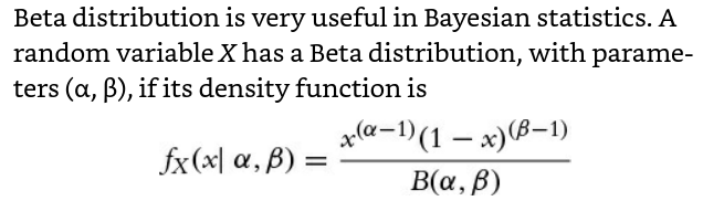
Beta(1,1) is the uniform distribution: thus Beta is a generalization of the uniform distribution.

Binomial and Beta distributions are connected: a Beta prior with binomial observations creates a Beta posterior: if we start with a Beta(1,1) prior on p, observe data X ~ Binomial(N,p), then our posterior is Beta (1+X, 1+N-X). For example, if we observe X = 10 successes out of N = 25 trials, then our posterior for p is a Beta(1+10, 1+25-10) = Beta (11,16)

Multiarmed bandits

Suppose you are faced with $N$ slot machines (colourfully called multi-armed bandits). Each bandit has an unknown probability of distributing a prize (assume for now the prizes are the same for each bandit, only the probabilities differ). Some bandits are very generous, others not so much. Of course, you don’t know what these probabilities are. By only choosing one bandit per round, our task is devise a strategy to maximize our winnings.

Of course, if we knew the bandit with the largest probability, then always picking this bandit would yield the maximum winnings. So our task can be phrased as “Find the best bandit, and as quickly as possible”.

The task is complicated by the stochastic nature of the bandits. A suboptimal bandit can return many winnings, purely by chance, which would make us believe that it is a very profitable bandit. Similarly, the best bandit can return many duds. Should we keep trying losers then, or give up?

A more troublesome problem is, if we have found a bandit that returns pretty good results, do we keep drawing from it to maintain our pretty good score, or do we try other bandits in hopes of finding an even-better bandit? This is the exploration vs. exploitation dilemma.

Any proposed strategy is called an online algorithm (not in the internet sense, but in the continuously-being-updated sense), and more specifically a reinforcement learning algorithm. The algorithm starts in an ignorant state, where it knows nothing, and begins to acquire data by testing the system. As it acquires data and results, it learns what the best and worst behaviours are (in this case, it learns which bandit is the best).

Step-by-step debug exploration of Bayesian multiarmed bandit

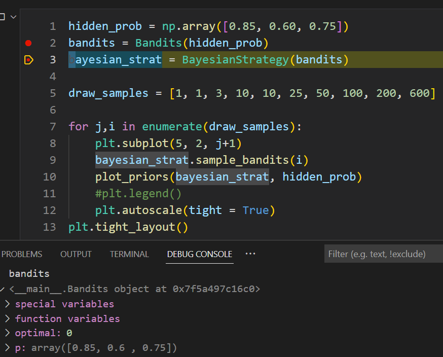
Here ‘bandits’ is such an object that contains array p, the hidden probabilities for each 3 bandits.

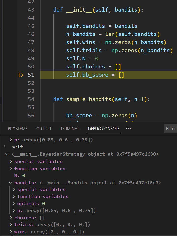
Nothing magical happens when the Bayesian strategy is initialized : it just stores the bandit and initializes some empty lists/arrays.

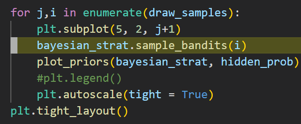
We start a loop and sample the bandits, first with i == 1

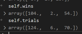
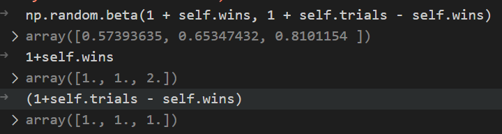
In the sample_bandits bit of implicit Python logic happening: because the self.wins and self.trials are length 3, the np.random.beta automatically returns three random values, one for each corresponging bandit

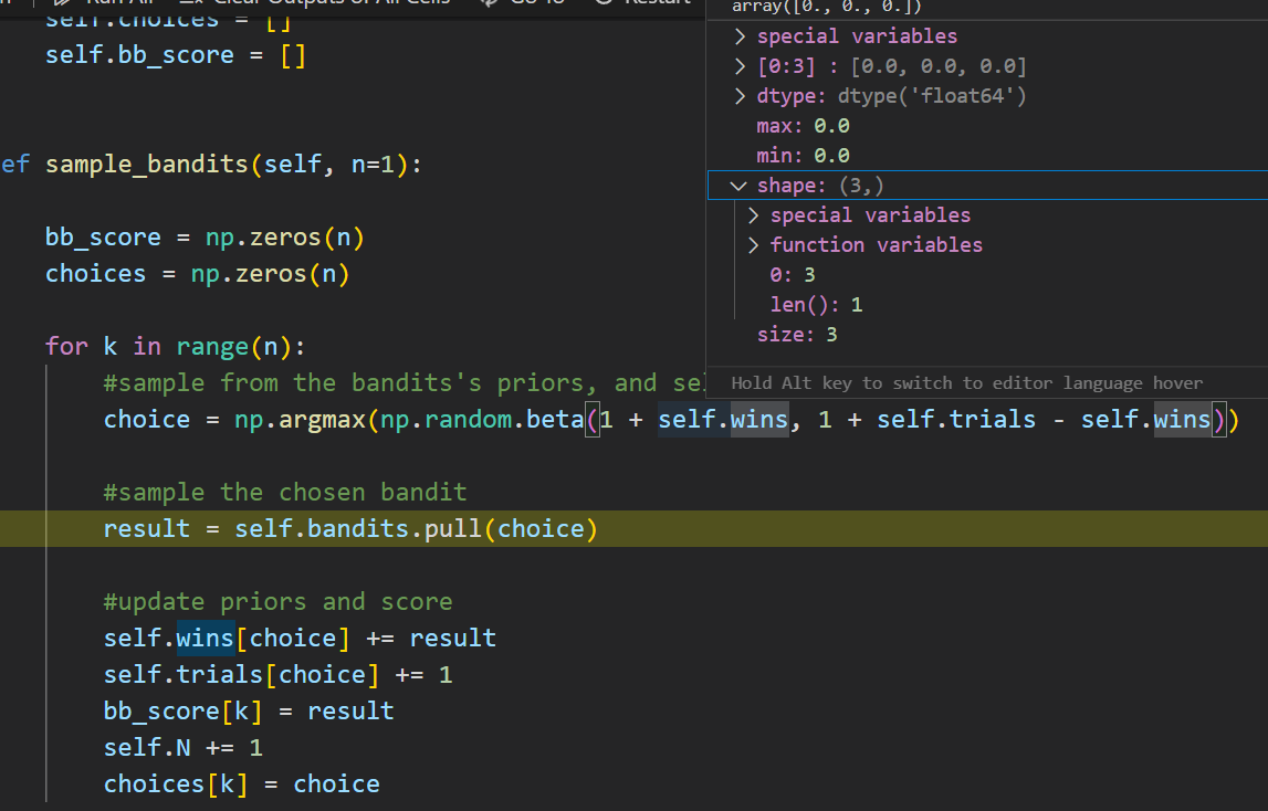
On the first run each bandit has the same probability to be chosen. On this debugging run the choice was 2 (thus the third bandit on 0-2 indexing). So that bandit is “pulled”

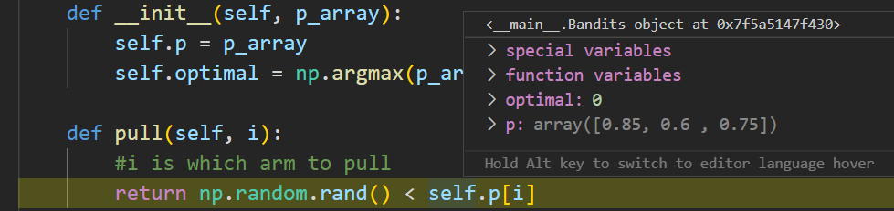
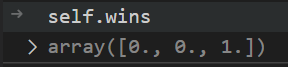
The hidden probability for third bandit is 0.75, so there is 75% chance that the pull is successful. The bandit returns this as success/failure. In this run, the bandit was successful so the bayesian strategy updates its memory:

On the next pull, the Beta distribution favors bandit 3 due to the previous success:

After 10 pulls the strategy is still very confused:

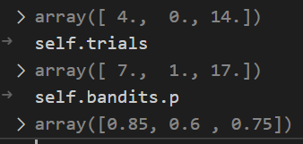
after couple hundred of pulls, the strategy has found that first bandit is the best, soemtimes favoring the third one, and completely ignoring the middle one: