PyMC in a nutshell (hopefully)
I’ve started to go through Rethinking Statistics book while systematically exploring how the models can be implemented not just in R but also PyMC and numpyro/jax. However, I realized that for this I should have at least reasonable understanding of PyMC and Numpyro. While I’ve studied both I can’t claim to be an expert, so before really starting the rethinking process a short detour to get the basics of these two frameworks.
I’ve also started using RemNote for memorizing stuff, so unfortunately some of the logs might go to remnote instead of here.
Pymc docs : https://www.pymc.io/projects/docs/en/latest/learn/core_notebooks/pymc_overview.html
While most of PyMC’s user-facing features are written in pure Python, it leverages Aesara (a fork of the Theano project) to transparently transcode models to C and compile them to machine code, thereby boosting performance. Aesara is a library that allows expressions to be defined using generalized vector data structures called tensors, which are tightly integrated with the popular NumPy ndarray data structure, and similarly allow for broadcasting and advanced indexing, just as NumPy arrays do. Aesara also automatically optimizes the likelihood’s computational graph for speed and allows for compilation to a suite of computational backends, including Jax and Numba.
# Following line creates a new Model object which is a container for the model random variables.
basic_model = pm.Model()


with basic_model:

    # Priors for unknown model parameters
    alpha = pm.Normal("alpha", mu=0, sigma=10)
    beta = pm.Normal("beta", mu=0, sigma=10, shape=2)
    sigma = pm.HalfNormal("sigma", sigma=1)

    # Expected value of outcome
    mu = alpha + beta[0] * X1 + beta[1] * X2

    # Likelihood (sampling distribution) of observations
    Y_obs = pm.Normal("Y_obs", mu=mu, sigma=sigma, observed=Y)
The final line of the model, defines Y_obs, the sampling distribution of the outcomes in the dataset.
This is a special case of a stochastic variable that we call an observed stochastic, and represents the data likelihood of the model. It is identical to a standard stochastic, except that its observed argument, which passes the data to the variable, indicates that the values for this variable were observed, and should not be changed by any fitting algorithm applied to the model. The data can be passed in the form of either a ndarray or DataFrame object.
The sample function runs the step method(s) assigned (or passed) to it for the given number of iterations and returns an InferenceData object containing the samples collected, along with other useful attributes like statistics of the sampling run and a copy of the observed data.
The PyMC Api (which is more concise)

logp is a method of the model instance. It puts together a function based on the current state of the model or on the state given as argument to logp.
Unobserved Random Variables
Every unobserved RV has the following calling signature: name (str), parameter keyword arguments. Thus:
with pm.Model():
    x = pm.Normal("x", mu=0, sigma=1)
Observed RV
with pm.Model():
    obs = pm.Normal("x", mu=0, sigma=1, observed=rng.standard_normal(100))
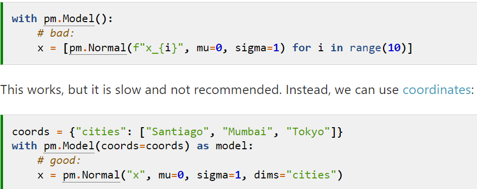
Multidim RV
Inference
sample() for MCMC and fit() for variational inference