Studies of nlp
To recap, let’s take a look at the final pipeline for the simple bag-of-words model. I want to emphasize that this model is only the start of our journey in feature extraction using NLP. We performed the following steps for normalization:
- Tokenization
- Removing punctuation marks
- Removing stop words
- Stemming
- Lemmatization with POS tagging
N and skip-grams
An n-gram is a concatenation of N consecutive entities
A, B, C, D -> 1-Gram: A, B, C, D
A, B, C, D -> 2-Gram: AB, BC, CD
A, B, C, D -> 3-Gram: ABC, BCD
We can extend the concept of n-grams to also allow the model to skip words. This a great option, if we for example want to perform a 2-gram, but in one of our samples there is an adjective in-between two words and in the other those words are directly next to each other. To achieve this, we need a method that allows us to define how many words it is allowed to skip to find matching words.
Reducing word dictionary size using SVD A common problem with NLP is the vast number of words in a corpus and, hence, exploding dictionary sizes. In the previous example, we saw that the size of the dictionary defines the size of the orthogonal term vector. Therefore, a dictionary size of 20,000 terms would result in 20,000-dimensional feature vectors. Even without any n-gram enrichment, this feature vector dimension is too large to be processed on standard PCs.
Therefore, we need an algorithm to reduce the dimensions of the generated CountVectorizer while preserving the present information. Optimally, we would only remove redundant information from the input data and project it onto a lower-dimensional space while preserving all of the original information.
The PCA transformation would be a great fit for our solution and help us to transform the input data into lower linearly unrelated dimensions. However, computing the eigenvalues requires a symmetric matrix (the same number of rows and columns), which, in our case, we don’t have. Hence, we can use the SVD algorithm, which generalizes the eigenvector computation to non-symmetric matrices. Due to its numeric stability, it is often used in NLP and information retrieval systems.
The usage of SVD in NLP applications is also called Latent Semantic Analysis (LSA), as the principal components can be interpreted as concepts in a latent feature space. The SVD embedding transforms the high-dimensional feature vector into a lower-dimensional concept space. Each dimension in the concept space is constructed by a linear combination of term vectors. By dropping the concepts with the smallest variance, we also reduce the dimensions of the resulting concept space to something that is a lot smaller and easier to handle. Typical concept spaces have 10s to 100s of dimensions, while word dictionaries usually have over 100,000.
from sklearn.decomposition import TruncatedSVD
svd = TruncatedSVD(n_components=5)
X_lsa = svd.fit_transform(X_train_counts)
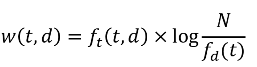
instead of an absolute count of terms in a context, we want to compute the number of terms in the context relative to a corpus of documents. By doing so, we will give higher weight to terms that appear only in a certain context, and reduce the amount of weight given to terms that appear in many different documents. This is exactly what the TF-IDF algorithm does. It is easy to compute a weight (w) for a term (t) in a document (d) according to the following equation:
In the following example, we will not use the TF-IDF function directly. Instead, we will use TfidfVectorizer, which does the counting and then applies the TF-IDF function to the result in one step. Again, the function is implemented as a sklearn transformer, and hence, we call fit_transform() to train and transform the dataset:
from sklearn.feature_extraction.text import TfidfVectorizer
vect = TfidfVectorizer()
data = [" ".join(words)]
X_train_counts = vect.fit_transform(data)
print(X_train_counts)
In any real-world pipeline, we would always use all the techniques presented in this chapter—tokenization, stop word removal, stemming, lemmatization, n-grams/skip-grams, TF-IDF, and SVD—combined in a single pipeline. The result would be a numeric representation of n-grams/skip-grams of tokens weighted by importance and transformed into a latent semantic space. Using these techniques for your first NLP pipeline will get you quite far, as you can now capture a lot of information from your textual data.