Stanford - Karpathy
https://www.youtube.com/watch?v=XfpMkf4rD6E
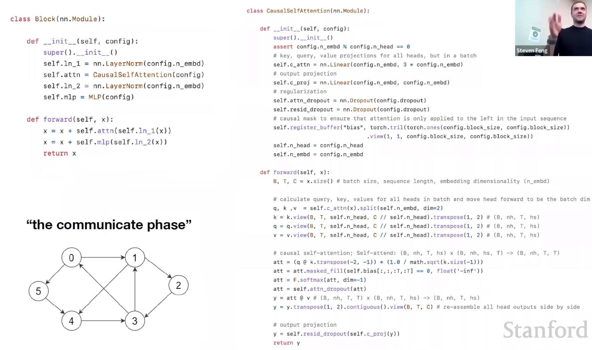
Coursera again
Adding an attention layer to this model avoids this problem by giving the decoder access to all parts of the input sentence. To illustrate, let’s just use a 4-word input sentence as shown below. Remember that a hidden state is produced at each timestep of the encoder (represented by the orange rectangles). These are all passed to the attention layer and each are given a score given the current activation (i.e. hidden state) of the decoder. For instance, let’s consider the figure below where the first prediction “Wie” is already made. To produce the next prediction, the attention layer will first receive all the encoder hidden states (i.e. orange rectangles) as well as the decoder hidden state when producing the word “Wie” (i.e. first green rectangle). Given this information, it will score each of the encoder hidden states to know which one the decoder should focus on to produce the next word. As a result of training, the model might have learned that it should align to the second encoder hidden state and subsequently assigns a high probability to the word “geht”. If we are using greedy decoding, we will output the said word as the next symbol, then restart the process to produce the next word until we reach an end-of-sentence prediction.
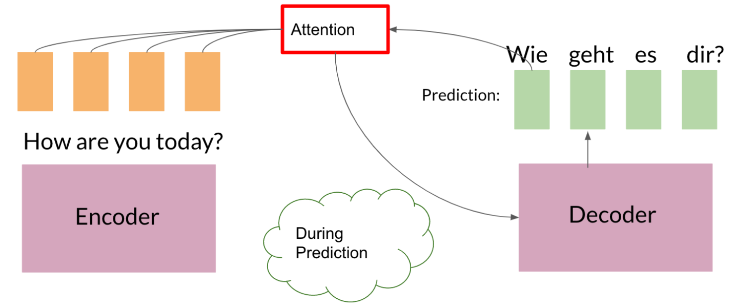
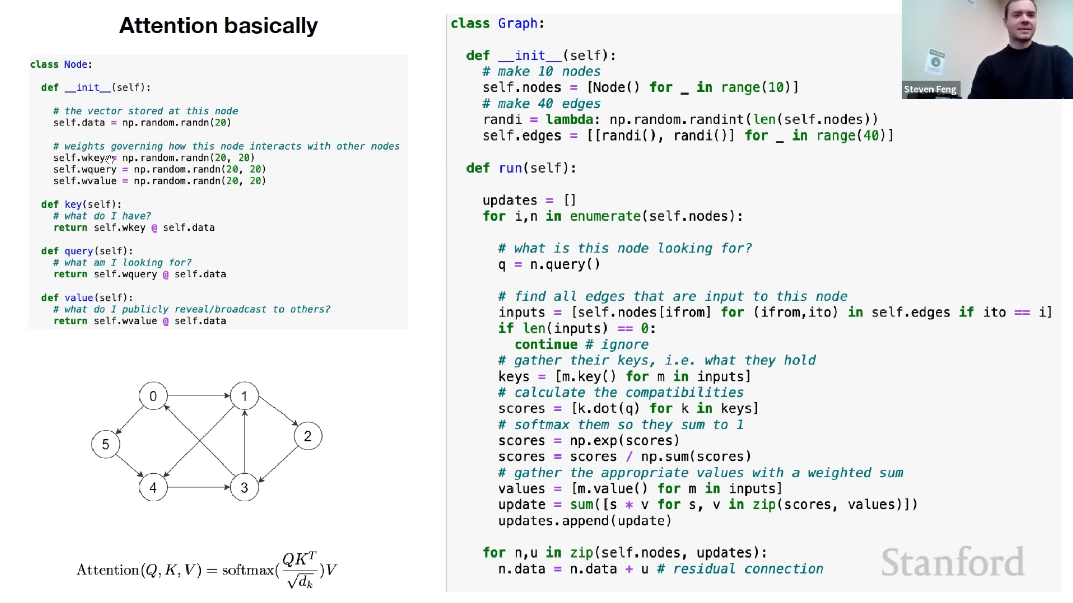
you can think of it as computing scores using queries (Q) and keys (K), followed by a multiplication of values (V) to get a context vector at a particular timestep of the decoder. This context vector is fed to the decoder RNN to get a set of probabilities for the next predicted word. The division by square root of the keys dimensionality is for improving model performance and you’ll also learn more about it next week. For our machine translation application, the encoder activations (i.e. encoder hidden states) will be the keys and values, while the decoder activations (i.e. decoder hidden states) will be the queries.