MCMC
Lots of stuff in the PyMC, Pyro etc pages. Now diving into MCMC from the Bayesian methods for hacker’s book
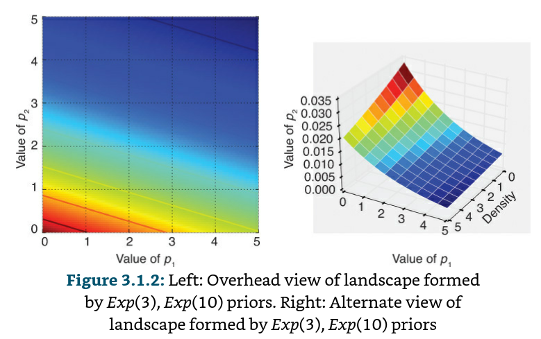
When we set up a Bayesian inference problem with N-unknowns, we are implicitly creating an N-dimensional space for the prior distributions to exist in. Associated with the space is an additional dimension, which we can describe as the surface, or curve, that sits on top of the space, that reflects the prior probability of a particular point. The surface on the space is defined by our prior distributions.

If these surfaces describe our prior distributions on the unknowns, what happens to our space after we incorporate our observed data X? The data X does not change the space, but it changes the surface of the space by pulling and stretching the fabric of the prior surface to reflect where the true parameters likely live. More data means more pulling and stretching, and our original surface may become mangled or insignificant compared to the newly formed surface. Less data, and our original shape is more present. Regardless, the resulting surface describes the new posterior distribution.
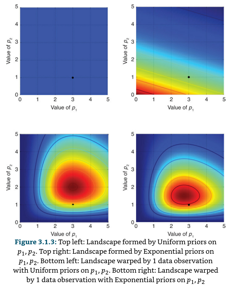
Suppose we are interested in performing inference on two Poisson distributions, each with an unknown λ parameter. We’ll compare using both a Uniform prior and an Exponential prior for the λ unknowns. Suppose we observe a data point; we visualize the “before” and “after” landscapes

The black dot in each of the four figures represents the true parameters. The plot on the bottom left is the deformed landscape with the Uniform(0, 5) priors, and the plot on the bottom right is the deformed landscape with the Exponential priors. Notice that the posterior landscapes look different from one another, though the data observed is identical in both cases. The reason is as follows. Notice that the posterior with the exponential-prior landscape, bottom-right figure, puts very little posterior weight on values in the upper-right corner of the figure; this is because the prior does not put much weight there. On the other hand, the Uniform-prior landscape is happy to put posterior weight in the upper-right corner, as the prior puts more weight there compared to the Exponential prior. Notice also that the highest point, corresponding to the darkest red, is biased toward (0,0) in the Exponential prior case, which is the result of the Exponential prior putting more prior weight in the (0,0) corner. Even with 1 sample point, the mountains attempt to contain the true parameter.
Explore the space with MCMC
We should explore the deformed posterior space generated by our prior surface and observed data to find the posterior mountain. However, we cannot naively search the space.
Recall that MCMC returns samples from the posterior distribution, not the distribution itself. Stretching our mountainous analogy to its limit, MCMC performs a task similar to repeatedly asking “How likely is this pebble I found to be from the mountain I am searching for?” and completes its task by returning thousands of accepted pebbles in hopes of reconstructing the original mountain. In MCMC and PyMC lingo, the “pebbles” returned in the sequence are the samples, cumulatively called the traces.
Unsupervised clustering example

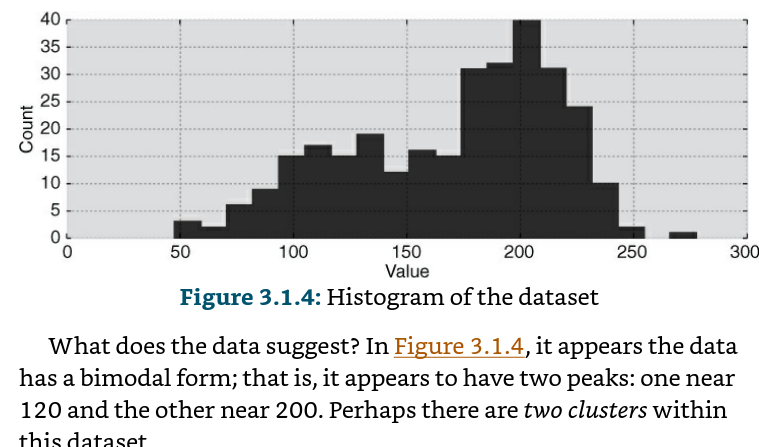
We can propose how above data might have been created:
- For each data point, choose cluster 1 with probability p, else choose cluster 2
- Draw a random variate from a Normal distribution with parameters $\mu_{i}$ and $\sigma_{i}$
- repeat
This algorithm would create a similar effect as the observed dataset, so we choose this as our model. Of course, we do not know p or the parameters of the Normal distributions. Hence we must infer, or learn, these unknowns. Denote the Normal distributions Nor0 and Nor1 (having variables’ index start at 0 is just Pythonic). Both currently have unknown mean and unknown standard deviation, denoted μi and σi, i = 0, 1 respectively. A specific data point can be from either Nor0 or Nor1, and we assume that the data point is assigned to Nor0 with probability p. A priori, we do not know what the probability of assignment to cluster 1 is, so we create a uniform variable over 0 to 1 to model this. Call this p.
import pymc as pm
 p = pm.Uniform("p", 0., 1.)
 assignment = pm.Categorical("assignment",[p, 1 - p], size=data.shape[0])