Statistic Rethinking Learning Journal
Chap 1.2
Chapter 3
3.3.2.2
We need to combine sampling simulated observations with sampling parameters from the posterior distribution: there is a lot of information about uncertainty in the entire posterior distribution. We lose this information when we pluck out single paramer value and then perform calculations iwht it. This loss of information leads to overconfidence.
First, there is observiation uncertainty. For any unique value of the parameter p, there is a unique implied pattern of observations that the model expects. There is uncertainty in the predicted observations because even if you know p with certainty, you won’t know the next toss…
Second, the re is uncertainty about p. The posteiror distribution over p embodies this uncertainty. And since there is uncertainty about p, there is uncertainty about everything that depends upon p.
We’d like to propagate the parameter uncertainty as we evaluate the implied predictions. All that is required is averaging over the posterior denstiy for p -> POSTERIOR PREDICTIVE DISTRIBUTION
To simulate predicted observations for a single value of p, say 0.6, we can use rbinom:
w <- rbinom(1e4, size=9, prob=0.6)
This generates 10k simulated predictions of 9 globe tosses assuming p is 0.6
Now we don’t just use one p but propagate the whole distribution:
w <- rbinom(1e4, size=9, prob=0.6)
Chapter 4
4.3 Gaussian model of height
Two parameters describingg the distribution shape, mean mu and std sigma. Bayesian updating will allow us to consider every possible combination of values for mu and sigma and to score each combination by its relative plausibility, in light of the data. These relative plausibilities are the posterior probabilities of each combination of values mu,sigma.
Prior Predictive simulation
essential part of modeling. Once the priors are chosen its important to check what they imply
Following the lecture.
First looking at the simpler model
We’ll fit a simple Gaussian model in Pymc3:

to sample from the model in Pymc3

the sample method returns a MultiTrace object from which we can extract samples :
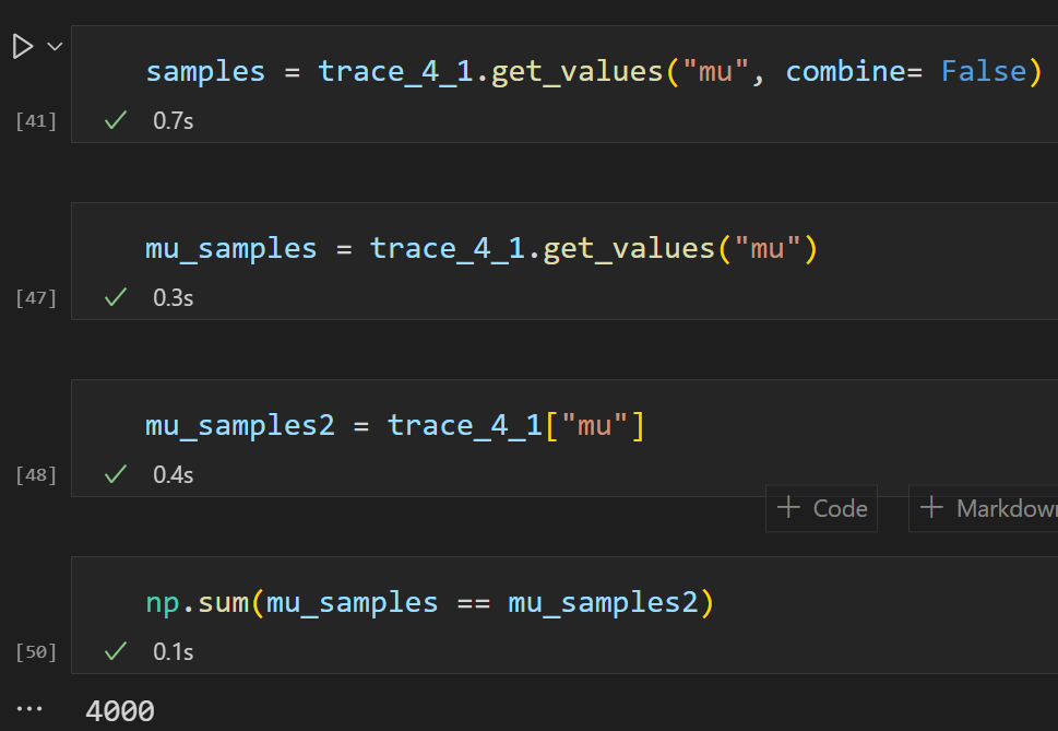
You can also play around with the initialization but I need to study more before starting to manually fiddle this:

Doing it in NumPyro:
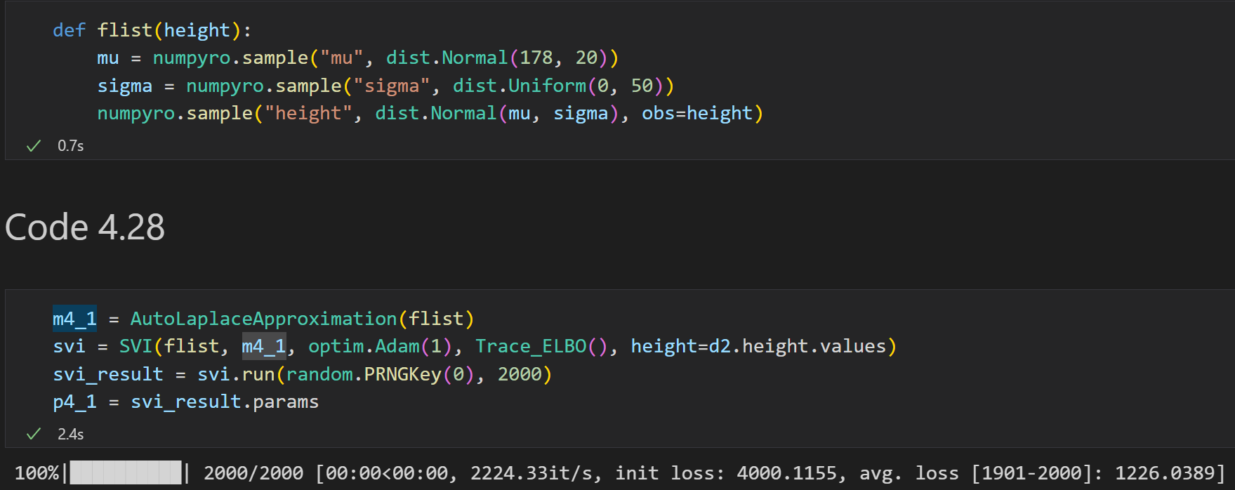
and we can get the posterior:

Same in R

we can use quadratic approximation to get the marginal distribution for each parameter. This means the plausibility of each value of mu, after averaging over the plausibilities of each of sigma.

Linear model: weight and height
To create and plot some priors in R
To get a posterior distribution using PyMC:

Link func
Generating predictions and intervals from the posterior of a fit model:
- Use link to generate distributions of posterior values for mu. The default behavior of link is to use the original data, so you have to pass it a list of new horizontal axis values you want to plot posterior predictions across.
- Use summary functions like mean or PI to find averages and lower and upper bounds of mu for each value of the predictor variable
- Finally, use plotting functions to draw the lines and intervals, or do calculations with them etc.
The link function uses the formula used to fit the model to compute the value of the linear model. It does this for each sample from the posterior distribution, for each case in the data. Here is a R version:
# After the following line we have 10k 3 dim samples in post for a,b and sigma
post <-extract.samples(m4.3)
mu.link <- function(weight) post$a + post$b*weight
weight.seq <- seq( from=25 , to=70 , by=1 )
# After the following we git 10k mean (mu) values for each weight specified in weight.seq
mu <- sapply( weight.seq , mu.link )
mu.mean <- apply( mu , 2 , mean )
mu.HPDI <- apply( mu , 2 , HPDI , prob=0.89 )
Same in numpyro/jax
post = m4_3.sample_posterior(random.PRNGKey(1), p4_3, (1000,))
mu_link = lambda weight: post["a"] + post["b"] * (weight - xbar)
weight_seq = jnp.arange(start=25, stop=71, step=1)
mu = vmap(mu_link)(weight_seq).T
mu_mean = jnp.mean(mu, 0)
mu_HPDI = hpdi(mu, prob=0.89, axis=0)
Prediction Intervals
Generating 89% prediction intervals for actual heights, not just the average height, $\mu$. This means we’ll incorporate the std $\sigma$ and its uncertaint as well
remember :
$h_{i} \sim$ Normal($\mu_{i}, \sigma$)
So far we have used just samples from the posterior to visualize the uncertainty in $\mu_{i}$, the linear model of the mean. But actual predictions of heights depend also upon the distribution in the first line.
imagine simulating heights. For any unique weight value, you sanmple from a Gaussian distribution with the correct mean $\mu$ for that weight, using the correct value of $\sigma$ sampled from the same posterior distribution. If you do this for every sample from the posterior, for every weight value of interest, you end up with a collection of simulated heights that embody the uncertainty in the posterior as well as the uncertainty in the Gaussian distribution of heights. Tool called sim does this
sim.height <- sim(m4.3, data=list(weight=weight.seq))
we get thousand samples for each 46 weights in weight.seq, but these are simulated heights, not distributions of plausible average height, $\mu$.
In numpyro:
sim_height = Predictive(m4_3.model, post, return_sites=["height"])( random.PRNGKey(2), weight_seq, None)["height"]
sim_height.shape, list(sim_height[:5, 0])
# outputs:
((1000, 46),
 [DeviceArray(135.85771, dtype=float32),
  DeviceArray(137.52162, dtype=float32),
  DeviceArray(133.89777, dtype=float32),
  DeviceArray(138.14607, dtype=float32),
  DeviceArray(131.1664, dtype=float32)])
In PyMC we only need one line of code:
height_pred = pm.sample_posterior_predictive(trace_4_3, 200, m4_3)
Two types of uncertainty
Above we encountered both uncertainty in parameter values (posterior) and uncertainty in a sampling process (posterior predictive).
- The posterior distribution is a ranking of the relative plausibilities of every possible combination of paramter values
- the distribution of simulated outcomes, like height, is instead a distribution that includes sampling variation from some process that generates Gaussian random variables.
4.5 Polynomials and splines
Doing polynomial regression is simple: just create a new variable that is the square of the previous predictor. Its good idea to standardize the values to not get too large.
d["weight_std"] = (d.weight - d.weight.mean()) / d.weight.std()
d["weight_std2"] = d.weight_std ** 2

with pm.Model() as m_4_5:
    a = pm.Normal("a", mu=178, sd=100)
    b1 = pm.Lognormal("b1", mu=0, sd=1)
    b2 = pm.Normal("b2", mu=0, sd=1)
    sigma = pm.Uniform("sigma", lower=0, upper=50)
    mu = pm.Deterministic("mu", a + b1 * d.weight_std + b2 * d.weight_std2)
    height = pm.Normal("height", mu=mu, sd=sigma, observed=d.height)
    trace_4_5 = pm.sample(1000, tune=1000)
Chapter 5
We are dealing with the following model/dag:
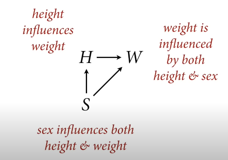
Deep dive into height / weight problem

Counterfactual plots
The basic recipe:
- Pick a variable to manipulate, the intervention variable
- Define the range of values to set the intervention variable to.
- For each value of the intervention variable, and for each sample in posterior, use the causal model to simulate the values of other variables, including the outcome.
Here is the marriage / divorce model in R:
data(WaffleDivorce)
d <- list()
d$A <- standardize( WaffleDivorce$MedianAgeMarriage )
d$D <- standardize( WaffleDivorce$Divorce )
d$M <- standardize( WaffleDivorce$Marriage )

m5.3_A <- quap(
    alist(
      ## A -> D <- M
        D ~ dnorm( mu , sigma ) ,
        mu <- a + bM*M + bA*A ,
        a ~ dnorm( 0 , 0.2 ) ,
        bM ~ dnorm( 0 , 0.5 ) ,
        bA ~ dnorm( 0 , 0.5 ) ,
        sigma ~ dexp( 1 ),
      ## A -> M
        M ~ dnorm( mu_M , sigma_M ),
        mu_M <- aM + bAM*A,
        aM ~ dnorm( 0 , 0.2 ),
        bAM ~ dnorm( 0 , 0.5 ),
        sigma_M ~ dexp( 1 )
    ) , data = d )
And in PyMC:
data["Divorce_std"] = standardize(data["Divorce"])
data["Marriage_std"] = standardize(data["Marriage"])
data["MedianAgeMarriage_std"] = standardize(data["MedianAgeMarriage"])

# Use Theano shared variables so we can change them later
marriage_shared = shared(data["Marriage_std"].values)
age_shared = shared(data["MedianAgeMarriage_std"].values)

with pm.Model() as m5_3_A:
    # A -> D <- M
    sigma = pm.Exponential("sigma", 1)
    bA = pm.Normal("bA", 0, 0.5)
    bM = pm.Normal("bM", 0, 0.5)

    a = pm.Normal("a", 0, 0.2)
    mu = pm.Deterministic("mu", a + bA * age_shared + bM * marriage_shared)
    divorce = pm.Normal("divorce", mu, sigma, observed=data["Divorce_std"])

    # A -> M
    sigma_M = pm.Exponential("sigma_m", 1)
    bAM = pm.Normal("bAM", 0, 0.5)
    aM = pm.Normal("aM", 0, 0.2)
    mu_M = pm.Deterministic("mu_m", aM + bAM * age_shared)
    marriage = pm.Normal("marriage", mu_M, sigma_M, observed=data["Marriage_std"])

    m5_3_A_trace = pm.sample()
then we create a list of 30 values between -2 and 2 sd as the values for the intervention variable
A_seq <- seq( from=-2 , to=2 , length.out=30 )
Then we first simluated M (which is influenced by A), and then D based on A and M
A_seq = np.linspace(-2, 2, 50)

# With PyMC3 we have to simulate in each model separately

# Simulate the marriage rates at each age first
age_shared.set_value(A_seq)

with m5_3_A:
    m5_3_M_marriage = pm.sample_posterior_predictive(m5_3_A_trace)
We can also check the numerical summaries, for example difference in effect of marriage age 20 vs 30
## R code 5.23
# new data frame, standardized to mean 26.1 and std dev 1.24
sim2_dat <- data.frame( A=(c(20,30)-26.1)/1.24 )
s2 <- sim( m5.3_A , data=sim2_dat , vars=c("M","D") )
mean( s2$D[,2] - s2$D[,1] )
The trick with simulating counterfactuals is to realize that when we manipulate some variable X, we break the causal influence of other variables on X. That is the same as saying we modify the DAG so that no arrows enter X. So in our marriage graph, if we manipulate M we break the A -> M path.
Overthinking counterfactual simulation
The example used sim() but simulating counterfactuals manually is not hard. Assume we’ve already fit the model m5.3_A above, the model that includes both causal paths A->D and A->M->D . We define again a range of values we want to assign to A:
A_seq <- seq( from=-2 , to=2 , length.out=30 )
Next we need to extract the posterior samples, because we’ll simulate observations for each set of samples. Then it really is just a matter of using the model definition with the samples. The model defines the distribution of M. We just convert that definition to the corresponding simulation function (rnorm in this case):
## R code 5.26
post <- extract.samples( m5.3_A )
M_sim <- with( post , sapply( 1:30 ,
    function(i) rnorm( 1e3 , aM + bAM*A_seq[i] , sigma_M ) ) )
above post is the posterior distribution over 7 variables:

and rnorm generates 1e3 samples for each , here for the first one:

So, after this we have in M_sim 1000 samples for each 30 points in A_seq.
After that we just use these values to simulate D:
## R code 5.27
D_sim <- with( post , sapply( 1:30 ,
    function(i) rnorm( 1e3 , a + bA*A_seq[i] + bM*M_sim[,i] , sigma ) ) )
now if we plot A_seq against D_sim we get the same counterfactual plot.
Simulating masking relationship
Categorical variables
Chapter 7
Two fundamental types of statistical error:
- The many-headed best of OVERFITTING, which leads to poor prediction by learning too much from the data
- the whirlpool of UNDERFITTING, which leads to poor prediction by learning too little from the data
- (and also confounding)
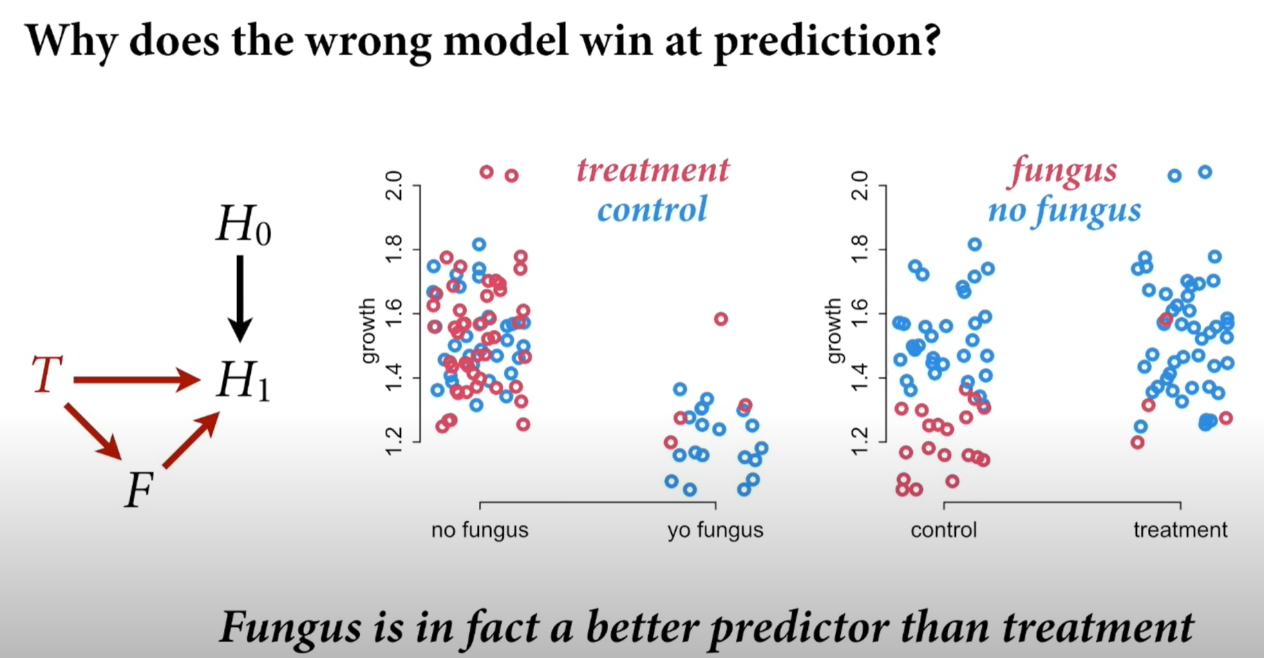
Confounded models can in fact produce better predictions than models that correctly measure a causal relationship.
the two solutions
- REGULARIZING PRIORS (or penalized likelihood in frequentist terminology)
- INFORMATION CRITERIA or CROSS-VALIDATION
If you are only interested in prediction and not causality, can you add all predictors: answer is no. leads to overfitting
Entropy and Accuracy
Path to out-of-sample deviancy
- establish a measurement scale for distance from perfect accuracy
- establish a deviance as an approximation of relative distance from perfect accuracy.
- establish that it is only deviance out-of-sample that is of interest.
Good measure for accuracy is the joint probability which is often log log prob.
So we want to use the log probability of the data to score the accuracy of competing models. The next problem is to measure the distance from perfect prediction.
Getting to the answer depends upon appreciating what an accuracy metric needs to do. It should appreciate that some targets are just easier to hit than other targets. For example, suppose we extend the weather forecast into the winter. Now there are three types of days: rain, sun, and snow. Now there are three ways of being wrong, instead of do (like in summer when it can either rain or be sunny). This has to be taken into account in any reasonable measure of distance from the target, because by adding another type of event, the target has gotten harder to hit.
It’s like taking a two-dimensional archery bullseye and forcing the archer to hit the target at the right time - a third dimension - as well. Now the possible distance between the best archer and the worst archer has grown, because there’s another way to miss. And with another way to miss, one might also say there is another way for an archer to timpress. As the potential distance between the target and the shot increases, so too does the potential improvement and ability of a talented archer to impress us.
The basic idea is to ask: How much is our uncertainty reduced by learning an outcome?
In the forecast context, forecasts are issued in advance and the weather isuncertain. When the actual day arrives, the weather is no longer uncertain. The reduction in uncertainty is then a natural measure of how much we have learned, how much “information” we derive from observing the outcome. So if we can develop a precise definition of “uncertainty,” we can provide a baseline measure of how hard it is to predict, as well as how much improvement is possible. The measured decrease in uncertainty is the definition of INFORMATION in this context.
INFORMATION ENTROPY
$H(p) = - E log(p_{i}) = - \sum_{i=1}^n p_{i} log(p_{i})$
MAXIMUM ENTROPY
Maximum entropy is a family of techniques for finding probability distributions that are most consistent with states of knowledge. In other words, given what we know, what is the least surprising distribution? It turns out that one answer to this question maximizes the information entropy, using the prior knowledge as constraint. If you do this, you actually end up with the posterior distribution. So Bayesian updating is entropy maximization.
From Entropy to Accuracy
Divergence:
The additional uncertainty induced by using probabilities from one distribution to describe another distribution. (Kullback-Leibler divergence)
The average difference in log probability between the target(p) and model(q)
What divergence can do for us now is help us contrast different approximations to p. As an approximating function q becomes more accurate D(p,q) will shring. So if we have a pair of candidate distributions, then the candidate that minimizes the divergence will be closest to the target. Since preditive models specify probabilities of events, we can use divergence to compare the accuracy of models.
Toe use $D_{KL}$ to compare models, it seems like would have to know p, the target probability, which is the thing we are trying to find. But there is a trick: we can compare two candidates for true probability instead, and see which one is closer.
So, we can just compare the average log-probability from each model to get an estimate of the relative distance of each model from the target.
Regularization
The root of overfitting is a model’s tendency to get overexcited by the training sample. When the priors are flat or nearly flat, the machine interprets this to mean that every parameter value is equally plausible. As a result, the model returns a posterior that encodes as much of the training sample - as represented by the likelihood functions - as possible.
One way to prevent this is to use a sceptial prior, a prior that slows the rate of learning, such as the regularizing prior.
AIC
For OLS regression with flat priors, the expected overfitting penatly is about twice the number of parameters. This phenomenom is behind INFORMATION CRITERIA, for example AIC:
${AIC = D_{train} + 2p = -2lppd +2p}$
AIC has some limitations and usually we use something like DIC or Widely Applicable Information Criterion WAIC that is more general. However, WAIC has problems with for example time-series!!
WAIC Calculation
## R code 7.19
data(cars)
m <- quap(
    alist(
        dist ~ dnorm(mu,sigma),
        mu <- a + b*speed,
        a ~ dnorm(0,100),
        b ~ dnorm(0,10),
        sigma ~ dexp(1)
    ) , data=cars )
set.seed(94)
post <- extract.samples(m,n=1000)
now we have the posterior of the above simple regression in variable post. We then get the log-likelihood of each observation:
## R code 7.20
n_samples <- 1000
logprob <- sapply( 1:n_samples ,
    function(s) {
        mu <- post$a[s] + post$b[s]*cars$speed
        dnorm( cars$dist , mu , post$sigma[s] , log=TRUE )
    } )

## R code 7.21
n_cases <- nrow(cars)
lppd <- sapply( 1:n_cases , function(i) log_sum_exp(logprob[i,]) - log(n_samples) )

## R code 7.22
pWAIC <- sapply( 1:n_cases , function(i) var(logprob[i,]) )

## R code 7.23
-2*( sum(lppd) - sum(pWAIC) )

## R code 7.24
waic_vec <- -2*( lppd - pWAIC )
sqrt( n_cases*var(waic_vec) )
Short summary of chap 7 so far
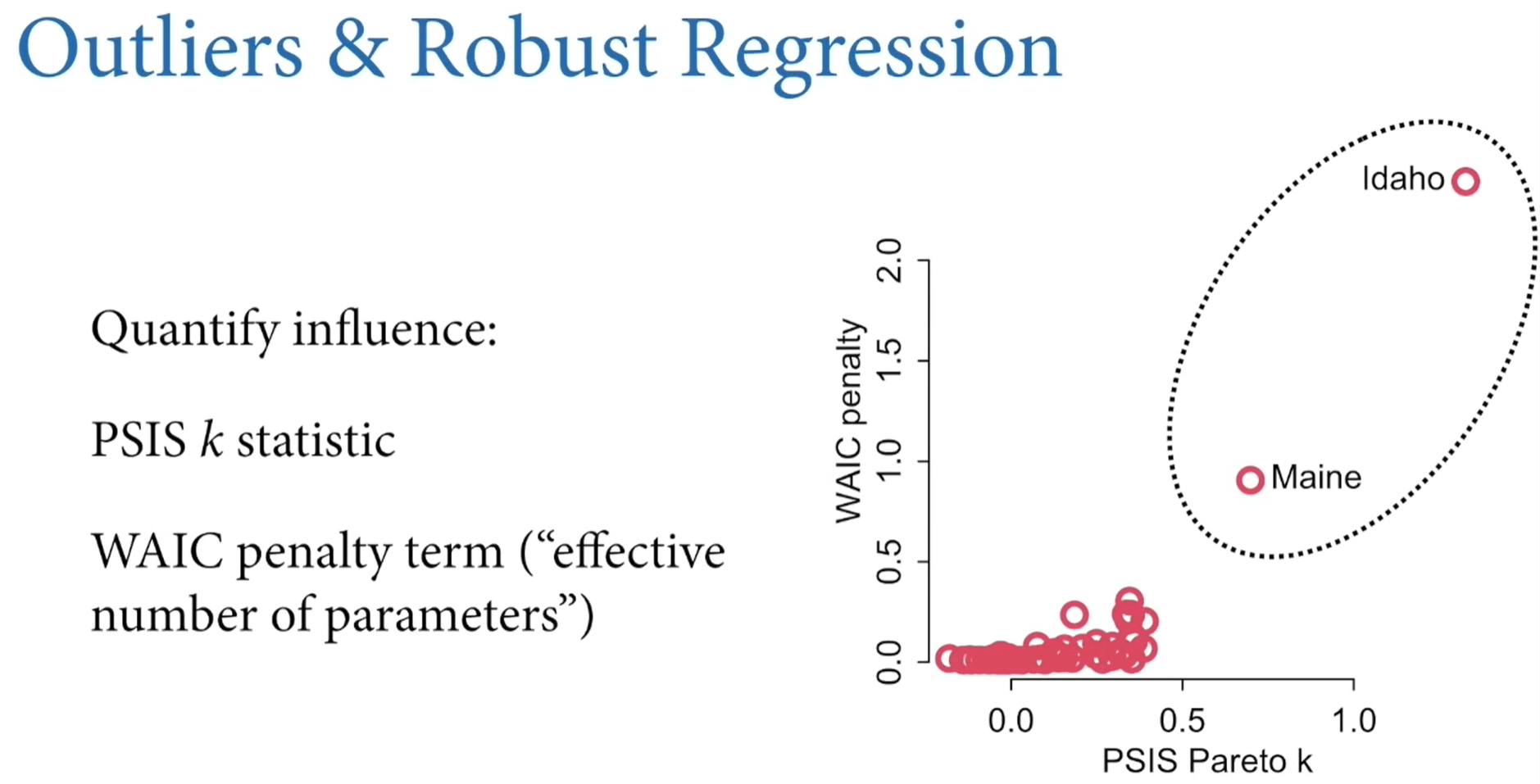
How to compare accuracy of models? Following fit to sample is no good as fit will always favor more complex models. Information divergence is the right measure of model accuracy, but it also prefers more complex models. We need to evaluate models out-of-sample: meta-model of forecasting tells us two important things:
- Flat priors produce bad predictions. Regularizing priors reduce fit to sample but tend to improve predictive accuracy.
- We can get a useful guess of predictive accuracy with criterias like CV, PSIS and WAIC which are complementary
Regularization reduces overfitting and predictive criteria measure it
When selecting models don’t just pick the one with lowest WAIC for two reasons:
- it discards the information about relative model accuracy which provides advie about how confident we might be about our models
- Maximizing predictive accuracy with WAIC does not care about causality (backdoor paths can improve predictive power)
So what good are these criteria then?
- they measure expected predictive value ofa variable on the right scale, accounting for overfitting. This helps in testing model implications given a set of causal models.
- they provide a way to measure the overfitting tendency of a mdoel, and that helps us both design models and understand how statistical inference works
- minimizing WAIR can help in designing models, especially in tuning parameters in multilevel models.
MODEL COMPARISON INSTEAD OF MODEL SELECTION
Causally incorrect but predictive models outperform causal ones in PSIS and WAIC scores

So, depending whether you are doing prediction (where you don’t care about causes) or causal modeling, you have to treat the values differently.
Chapter 9: MCMC
Metropolis algorithms
- The ‘islands’ in our objective are parameter values, and they need not be discrete
- The ‘population sizes’ in our objective are the posterior probabilities at each parameter value
- the ‘weeks’ in our objective are samples taken from the joint posterior of the parameters in the model
In basic metro the propositions to move are symmetric (left and right ‘island’ has equal probability), asymmetric version is known as Metropolis-Hasting.
Gibbs Sampling
Gibbs sampling is a variant of the Metropolis-Hastings algorithm that uses clever proposals and is tehrefore more efficient. The improvement arises from adaptive proposals in which the distribution of proposed parameter vlaues adjusts itself intelligently, depending upon the parameter vlaues at the moment.
Gibbs needs conjugate pairs.
Concentration of Measure
The probability mass of a high-dimensional distribution is always very far from the mode of the distribution (its a ring at certain ‘height’)
Hamiltonian Monte Carlo
We use gradients to “flow” around
HMC overthought
The HMC algorithm needs five things to go:
- a function U that returns the negative log-probability of the data at the current position (parameter values)
- a function grad_U that returns the gradient of the negative log-probability at the current position
- a step size epsilon
- count of leapfrog steps L
- a starting position current
Example : Two Gaussians from Normal(0,1)
The U function:
# U needs to return neg-log-probability
U <- function( q , a=0 , b=1 , k=0 , d=1 ) {
    muy <- q[1]
    mux <- q[2]
    U <- sum( dnorm(y,muy,1,log=TRUE) ) + sum( dnorm(x,mux,1,log=TRUE) ) +
        dnorm(muy,a,b,log=TRUE) + dnorm(mux,k,d,log=TRUE)
    return( -U )
}
Gradient function
U_gradient <- function( q , a=0 , b=1 , k=0 , d=1 ) {
    muy <- q[1]
    mux <- q[2]
    G1 <- sum( y - muy ) + (a - muy)/b^2 #dU/dmuy
    G2 <- sum( x - mux ) + (k - mux)/d^2 #dU/dmux
    return( c( -G1 , -G2 ) ) # negative bc energy is neg-log-prob
}
The HMC2 function runs a single trajectory and thus produces a single sample.
HMC2 <- function (U, grad_U, epsilon, L, current_q) {
  q = current_q
  p = rnorm(length(q),0,1) # random flick - p is momentum.
  current_p = p
  # Make a half step for momentum at the beginning
  p = p - epsilon * grad_U(q) / 2
  # initialize bookkeeping - saves trajectory
  qtraj <- matrix(NA,nrow=L+1,ncol=length(q))
  ptraj <- qtraj
  qtraj[1,] <- current_q
  ptraj[1,] <- p

## R code 9.9
  # Alternate full steps for position and momentum
  for ( i in 1:L ) {
    q = q + epsilon * p # Full step for the position
    # Make a full step for the momentum, except at end of trajectory
    if ( i!=L ) {
        p = p - epsilon * grad_U(q)
        ptraj[i+1,] <- p
    }
    qtraj[i+1,] <- q
  }

## R code 9.10
  # Make a half step for momentum at the end
  p = p - epsilon * grad_U(q) / 2
  ptraj[L+1,] <- p
  # Negate momentum at end of trajectory to make the proposal symmetric
  p = -p
  # Evaluate potential and kinetic energies at start and end of trajectory
  current_U = U(current_q)
  current_K = sum(current_p^2) / 2
  proposed_U = U(q)
  proposed_K = sum(p^2) / 2
  # Accept or reject the state at end of trajectory, returning either
  # the position at the end of the trajectory or the initial position
  accept <- 0
  if (runif(1) < exp(current_U-proposed_U+current_K-proposed_K)) {
    new_q <- q  # accept
    accept <- 1
  } else new_q <- current_q  # reject
  return(list( q=new_q, traj=qtraj, ptraj=ptraj, accept=accept ))
}
Chapter 10: Entropy and GLM
When a researcher wants to build an unconventional model, entropy provides on useful principle to guide choice of probability distributions: best on the distribution with the biggest entropy. There are three reasons for this:
- The distribution with the biggest entropy is the widest and least informative distribution which means spreading probability as evenly as possible, while still remaining consistent with anything we thinkg we know about a process. In the context of choosing a prior, it means choosing the least informative distribution consistent with any partial scientific knowledge we have about a parameter. In the context of choosing a likelihood, it means selecting the distribution we’d get by counting up all the ways outcomes could arise, consistent with the contraints on the outcome variable.
- Nature tends to produce empirical distributions that have high entropy (like the Normal distribution)
- It just works.
Bayesian updating is entropy maximization
Posterior distribution deduced by Bayesian updating is also a case of maximizing entropy. The posterior distribution has the greatest entropy relative to the prior (the smallest cross entropy) among all distributions consistent with the assumed constraints and the observed data. Bayesian updating produces the least informative distribution that is still consistent with our assumptions; posterior ha the smallest divergence from the prior that is possible while remaining consistent with the constraints and data.
As we remember, the (unique) measure of the uncertainty of a probability distribution p whith probabilities $p_i$ for each possible event i turns out to be just the average log-probability, which is also information entropy
The principle of maximum entropy applies this measure of uncertainty to the problem of choosing among probability distributions:
The distribution that can happen the most ways is also the distribution with the biggest information entropy. The distribution with the biggest entropy is the most conservative distribution that obeys its contraints.
Information entropy is a way of counting how many unique arrangements correspond to a distribution. Remember the pebble example where 10 pebbles are divided in 10 buckets. Setup where each bucket has 2 pebbles can happen in most ways and thus has the highest entropy, while setup where all pebbles are in one bucket has the lowest.
The distribution that can happen the greatest number of ways is the most plausible distribution, and is called MAXIMUM ENTROPY DISTRIBUTION.
Binomial as max entropy
When only two un-ordered outcomes are possible and the expected numbers of each type of event are assumed to be constant, then the distribution that is most consistent with these constraints is the binomial distribution. This distribution spreads the probability out as evenly and conservatively as possible.
Second, of course usually we do not know the expected value, but wish to estimate it. But this is actually the same problem, because assuming the distribution has a constant expected value leads to the binomial distribution as well, but with unknown expected value np which must be estimated from teh data.
Histomancy: dicvining likelihood functions from empirical histograms
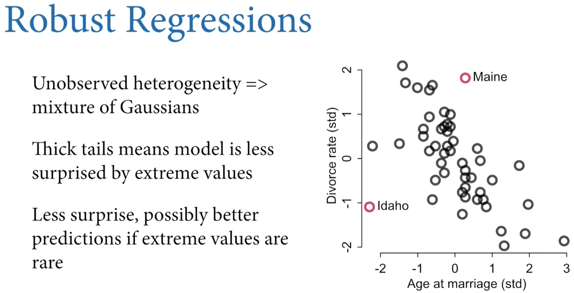
Bad idea! for example perfectly good Gaussian variables may not look Gaussian: at what a Guassian likelihood assumes is not that the aggregated data looks Gaussian, but rather that the residuals, after fitting the model, look Gaussian. So for example the combined histogram of male and female body weights is certainly not Gaussian. But its a mixture of Gaussian distribution, so after conditioning on sex, the residuals may be quite normal.
Exponential Family
Exponential distribution
Constrained to be zero or positive. It is a fundamental distribution of distance and duration, kinds of measurements that represent displacement from some point of reference, either in time or space. If the probability of an event is constant in time or across space, then the distribution of events tends towards exponential. Its shape is described by single parameter, the rate of events lambda.
Gamma Distribution
also constrained to be zero or positive. It too is a fundamental distribution of distance and duration. But unlike the exponential distribution, the gamma distribution can have a peak above zero. If an event can only happen after two or more exponentially distributed events happen, the resulting waiting times will be gamma distributed.
Poisson Distribution
is a count distribution like the binomial It is actually a special case of binomial. If the number of trials n is very large (and usually unknown) and the probability of a success p is very small, the a binomial distribution converges to a Poisson distribution with an expected rate of events per unit time of lambda = np.
Chapter : 16.2
Consider experiment in which 629 children aged 4 to 14 saw four other children choose among three different colored boxes. Each then them ade their own choice. In each trial, three demonstrators chose the same color. The fourth demonstrator chose a different color. So in each trial, one of the color was the majority choice, another was the minority choice, and the final color was unchosen. How do we figure out if children where influenced by teh majoirty